India’s central bank cut its policy repo rate for the 5th time this year, as expected, and said it would “continue with an accommodative stance as long a it is necessary to revive growth, while ensuring that inflation remains within the target.”
The Reserve Bank of India (RBI) cut the repo rate by another 25 basis points to 5.15 percent and has now cut it by a total of 135 points this year following cuts in February, April, June and August.
India’s economy has slowed in the last four quarters and the RBI again lowered its forecast for economic growth in the 2019-20 financial year, which began April 1, to 6.1 percent from 6.9 percent forecast in August, with the risks evenly balanced, down from 6.8 percent in 2018-19.
Gross domestic product in the first quarter of 2019-20, or the second calendar quarter, slowed to 5.0 percent year-on-year, well below RBI’s forecast range of 5.8-6.6 percent, amid weakening global growth and heightened uncertainty from trade and geopolitical tensions that cloud the outlook.
For the first quarter of next financial year, 2020-21, RBI also revised downwards its growth forecast to 7.2 percent from a previous 7.4 percent.
Although India’s government has announced a $20 billion tax cut, which should strengthen private consumption and private investment, and past rate cuts should gradually boost demand, RBI added “the continuing slowdown warrants intensified efforts to restore the growth momentum.”
“With inflation expected to remain below target in the remaining period of 2019-20 and Q1:2020-21, there is policy space to address these growth concerns by reinvigorating domestic demand within the flexible inflation targeting mandate,” RBI said.
India’s inflation rate rose for the 7th month in a row to 3.21 percent in August but remains below the RBI’s target of 4.0 percent, plus/minus 2 percentage points, but in line with its past forecast.
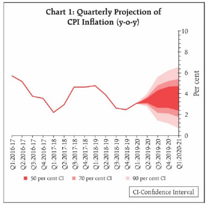
RBI revised slightly upward its forecast for headline inflation to 3.4 percent for the second quarter of 2019-20, and retained them at 3.5-3.7 percent for the second half of 2019-20, and 3.6 percent for the first quarter of 2020-21.
The Reserve Bank of India released its fourth bi-monthly monetary policy statement by its monetary policy committee, followed by a statement by its governor, Shaktikanta Das:
“On the basis of an assessment of the current and evolving macroeconomic situation, the Monetary Policy Committee (MPC) at its meeting today (October 4, 2019) decided to:
reduce the policy repo rate under the liquidity adjustment facility (LAF) by 25 basis points to 5.15 per cent from 5.40 per cent with immediate effect.
Consequently, the reverse repo rate under the LAF stands reduced to 4.90 per cent, and the marginal standing facility (MSF) rate and the Bank Rate to 5.40 per cent.
The MPC also decided to continue with an accommodative stance as long as it is necessary to revive growth, while ensuring that inflation remains within the target.
These decisions are in consonance with the objective of achieving the medium-term target for consumer price index (CPI) inflation of 4 per cent within a band of +/- 2 per cent, while supporting growth.
The main considerations underlying the decision are set out in the statement below.
Assessment
Global Economy
2. Since the MPC’s last meeting in August 2019, global economic activity has weakened further. Heightened uncertainty emanating from trade and geo-political tensions continues to cloud the outlook. Among advanced economies (AEs), the slowdown in the US economy in Q2:2019 appears to have extended into Q3:2019, weighed down by softer industrial production. The Institute for Supply Management’s index for September indicates that manufacturing slipped further into contraction to touch its lowest reading in a decade; hiring by the private sector also slowed down. In the Euro area too, incoming data suggest that activity may have moderated further in Q3, with retail sales declining and manufacturing PMI remaining in contraction for the eighth consecutive month in September. The UK economy decelerated in Q2; the contraction in industrial production and soft retail sales in July suggest that the loss of speed has continued into Q3 as well. In Japan, the loss of momentum in Q2 spilled over into Q3, albeit cushioned by a fiscal stimulus and frontloaded consumer spending ahead of a planned sales tax hike.
3. The macroeconomic performance of major emerging market economies (EMEs) was weighed down by a deteriorating global environment in Q3. The Chinese economy appears to have slowed down in Q3 as well, with both retail sales and industrial production growth weakening in July-August and exports contracting in August; attention is now focussed on the efficacy of fiscal and monetary policy stimuli in averting a sharper deceleration. In Russia, economic activity ticked up in Q2, though still subdued consumer sentiment and weak industrial production may restrain momentum, going forward. Economic activity in both South Africa and Brazil rebounded in Q2, emerging out of contraction in the previous quarter; however, this nascent recovery faces both domestic and external headwinds.
4. Crude oil prices were pulled down by softer demand, amidst adequate supplies in early August. Prices remained range bound until mid-September when supply disruptions on account of an escalating geo-political conflict resulted in a spike which has abated faster than expected. Gold prices remained elevated on safe haven demand. Central banks became more accommodative with inflation remaining below targets across major AEs and EMEs.
5. Global financial markets have remained unsettled since the MPC’s early August meeting with bouts of volatility unleashed by protectionist policies and worsening global growth prospects. In the US, the equity market’s August losses were recouped by early September – investor sentiment was buoyed by signs of an easing in US-China trade tensions. Stock markets in EMEs fell, as the strong US dollar led to capital outflows, though they recovered partially in September. Bond yields in the US continued easing till August on growth worries, before a slight uptick was triggered in early September by better than expected US retail sales data and hopes of conciliatory trade negotiations between the US and China. In the Euro area, bond yields sank further into negative territory, propelled by the cut in the deposit rate by the European Central Bank (ECB) to (-) 0.5 per cent and the reintroduction of quantitative easing. In EMEs, bond yields exhibited mixed movements, driven by country-specific factors. In currency markets, the US dollar strengthened against currencies of other AEs. EME currencies, which were trading with a depreciating bias in August, appreciated in early September on country-specific factors and a revival of global risk-on sentiment.
Domestic Economy
6. On the domestic front, growth in gross domestic product (GDP) slumped to 5.0 per cent in Q1:2019-20, extending a sequential deceleration to the fifth consecutive quarter. Of its constituents, private final consumption expenditure (PFCE) slowed down to an 18-quarter low. Gross fixed capital formation (GFCF) improved marginally on a sequential basis but remained muted as in the preceding quarter. Government final consumption expenditure (GFCE) cushioned the overall loss of momentum to some extent.
7. On the supply side, gross value added (GVA) growth decelerated to 4.9 per cent in Q1:2019-20, pulled down by manufacturing growth, moderating to 0.6 per cent. Agriculture and allied activities were lifted by higher production of wheat and oilseeds during the 2018-19 rabi season. Growth in the services sector was stalled by construction activity.
8. Turning to Q2:2019-20, the initial delay in the onset of the south-west monsoon rapidly caught up from July. By September 30, 2019, the cumulative all-India rainfall surpassed the long period average (LPA) by 10 per cent. The first advance estimates of major kharif crops for 2019-20 have placed production of foodgrains 0.8 per cent lower when compared with the last year’s fourth advance estimates. Looking ahead at the rabi season, the live storage of water in major reservoirs was 115 per cent of the live storage of the corresponding period of the previous year on September 26, 2019 and 121 per cent of average storage level over the last ten years. Abundant rains in August and September have led to improved soil moisture conditions in most parts of the country, particularly central India, compared to the corresponding period of the last year. Overall, the prospects of agriculture have brightened considerably, positioning it favourably for regenerating employment and income, and the revival of domestic demand.
9. Industrial activity, measured by the index of industrial production (IIP), weakened in July 2019 (y-o-y), weighed down mainly by moderation in manufacturing. In terms of uses, the production of capital goods and consumer durables contracted. Consumer non-durables, led by edible oils, and intermediate goods, mainly mild steel slabs, posted sustained expansion and have emerged as potential growth drivers. Infrastructure/construction sector activity turned around to register a growth of 2.1 per cent vis-à-vis (-)1.9 per cent in the previous month. The output of eight core industries contracted in August, pulled down by coal, electricity, crude oil and cement. Capacity utilisation (CU) in the manufacturing sector, measured by the OBICUS (order books, inventory and capacity utilisation survey) of the Reserve Bank, declined to 73.6 per cent in Q1:2019-20 from 76.1 per cent in the previous quarter. However, seasonally adjusted CU rose to 74.8 per cent in Q1:2019-20 from 74.5 per cent in Q4:2018-19. Manufacturing firms polled for the industrial outlook survey (IOS) expect capacity utilisation to moderate in Q2:2019-20. The Reserve Bank’s business assessment index (BAI) fell in Q2:2019-20 due to a decline in new orders, contraction in production, lower capacity utilisation and fall in profit margins of the surveyed firms. The manufacturing purchasing managers’ index (PMI) for September 2019 was unchanged at its previous month’s level; new orders and employment improved, albeit marginally, and new export orders declined.
10. High frequency indicators suggest that services sector activity weakened in July-August. Indicators of rural demand, viz., tractor and motorcycles sales, contracted. Of underlying indicators of urban demand, passenger vehicle sales contracted in July-August, while domestic air passenger traffic accelerated in August. The sales of commercial vehicles, a key indicator for the transportation sector, contracted by double digits in July-August. Of the two indicators of construction activity, finished steel consumption decelerated sharply in August and cement production contracted. The services PMI moved into contraction in September 2019, dragged down mainly by a decline in new business inflows.
11. Retail inflation, measured by y-o-y changes in the CPI, moved in a narrow range of 3.1- 3.2 per cent between June and August. While food inflation picked up, fuel prices moved into deflation. Inflation excluding food and fuel softened in August.
12. Food inflation in August was elevated by a spike in the rate of increase in vegetables prices, a pick-up in pulses inflation and persistently high meat and fish inflation. On the other hand, softer increases in prices of eggs, oils and fats, non-alcoholic beverages and prepared meals, and deflation in prices of fruits and sugar cushioned the rise in overall food inflation.
13. Deflation in the fuel group deepened in August largely due to the pass-through from a sharp decline in international prices of liquified petroleum gas (LPG). Subsidised kerosene prices, however, have been rising in a calibrated manner as oil marketing companies continued a gradual reduction in subsidies.
14. CPI inflation excluding food and fuel increased in July, but its roots were largely confined to prices of personal care and effects – mainly bullion prices, and transport and communication, reflecting rise in prices of petrol and diesel. By contrast, there was moderation in August, which was spread across most of the sub-groups; however, gold prices spiked further on global uncertainties.
15. The Reserve Bank’s September 2019 round of inflation expectations survey indicates that households expect inflation to rise by 40 basis points over a 3-month ahead horizon and 20 basis points over a one-year ahead horizon, possibly responding adaptively to the rise in food prices in recent months. The Reserve Bank’s consumer confidence survey shows weak consumer sentiment and tepid consumption demand, especially relating to non-essential items. Manufacturing firms see weakening of demand conditions in Q2:2019-20 and Q3 and expect their output prices to soften, going forward, as the cost of finance and salary outgoes remain muted.
16. Overall liquidity remained surplus in August and September 2019 despite expansion of currency in circulation and forex operations by the Reserve Bank draining liquidity from the system. Net daily average absorption under the LAF amounted to ₹1,40,497 crore in August, essentially on account of spending by the government, which resulted in availment of ways and means advances (WMA) and intermittent overdraft facilities from the beginning of the month (till August 25, 2019). In September, with a steady build-up of cash balances, particularly with advance tax inflows around September 15, surplus liquidity moderated, and the Reserve Bank undertook daily net absorption of ₹1,22,392 crore in September. Reflecting easy liquidity conditions, the weighted average call rate (WACR) traded below the policy repo rate (on an average) by 8 basis points (bps) in August and by 6 bps in September.
17. Monetary transmission has remained staggered and incomplete. As against the cumulative policy repo rate reduction of 110 bps during February-August 2019, the weighted average lending rate (WALR) on fresh rupee loans of commercial banks declined by 29 bps. However, the WALR on outstanding rupee loans increased by 7 bps during the same period.
18. Net exports had contributed to aggregate demand in Q1:2019-20 on account of a deeper contraction in imports relative to exports. In Q2, merchandise exports remained weak in July and August 2019, caused by lower shipments of engineering goods, petroleum products, gems and jewellery and cotton yarn. Imports contracted faster during the period mainly due to lower international crude oil prices downsizing the oil import bill and a large fall in the volume of gold imports. Non-oil non-gold imports were pulled down into contraction by coal, pearls and precious stones and transport equipment. These developments led to a narrowing of the trade deficit during July-August 2019. Higher net services receipts and private transfer receipts helped contain the current account deficit to 2.0 per cent of GDP in Q1:2019-20 from 2.3 per cent a year ago. On the financing side, net foreign direct investment rose to US$ 17.7 billion in April-July 2019 from US$ 11.4 billion a year ago. Net foreign portfolio investment (excluding the voluntary retention route) was of the order of US$ 3.3 billion during April-September 2019 as against net outflow of US$ 11.5 billion in the same period of last year. Net disbursals of external commercial borrowings rose to US$ 8.2 billion during April-August 2019 as against net repayments of US$ 0.2 billion during the same period a year ago. India’s foreign exchange reserves were at US$ 434.6 billion on October 1, 2019 – an increase of US$ 21.7 billion over end-March 2019.
Outlook
19. In the third bi-monthly resolution of August 2019, CPI inflation was projected at 3.1 per cent for Q2:2019-20, 3.5-3.7 per cent for H2:2019-20 and 3.6 per cent for Q1: 2020-21 with risks evenly balanced. The actual inflation outcomes for Q2 so far (July-August) at 3.2 per cent have been broadly in line with these projections.
20. Going forward, several factors are likely to shape the inflation trajectory. First, the outlook for food inflation has improved considerably since the August bi-monthly policy. Kharif production is estimated at close to last year’s level, auguring well for the overall food supply situation. Vegetable prices may remain elevated in the immediate months but are likely to moderate as winter supplies enter the market. Prices of pulses are expected to remain contained by adequate buffer stocks. Secondly, forward looking surveys conducted by the Reserve Bank point to weak demand conditions persisting, with indications of softening of output prices in Q3:2019-20. Accordingly, price pressures in CPI excluding food and fuel are likely to be muted. Thirdly, crude oil prices may remain volatile in the near-term; while global demand is slowing down, the persisting geo-political uncertainties pose some upside risks to the inflation outlook. Fourthly, three-month and one-year ahead inflation expectations of households polled by the Reserve Bank have risen in the current round reflecting near-term price pressures. Finally, financial markets remain volatile with currencies of several emerging market economies trading with a depreciating bias in the recent period. Taking into consideration these factors and the impact of recent policy rate cuts, the CPI inflation projection is revised slightly upwards to 3.4 per cent for Q2:2019-20, while projections are retained at 3.5-3.7 per cent for H2:2019-20 and 3.6 per cent for Q1:2020-21, with risks evenly balanced (Chart 1).
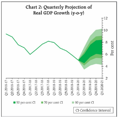
21. Turning to the growth outlook, real GDP growth for 2019-20 in the August policy was projected at 6.9 per cent – in the range of 5.8-6.6 per cent for H1:2019-20 and 7.3-7.5 per cent for H2 – with risks somewhat tilted to the downside; GDP growth for Q1:2020-21 was projected at 7.4 per cent. GDP growth for Q1:2019-20 was significantly lower than projected. Various high frequency indicators suggest that domestic demand conditions have remained weak. The business expectations index of the Reserve Bank’s industrial outlook survey shows muted expansion in demand conditions in Q3. Export prospects have been impacted by slowing global growth and continuing trade tensions. On the positive side, however, the impact of monetary policy easing since February 2019 is gradually expected to feed into the real economy and boost demand. Several measures announced by the Government over the last two months are expected to revive sentiment and spur domestic demand, especially private consumption. Taking into consideration the above factors, real GDP growth for 2019-20 is revised downwards from 6.9 per cent in the August policy to 6.1 per cent – 5.3 per cent in Q2:2019-20 and in the range of 6.6-7.2 per cent for H2:2019-20 – with risks evenly balanced; GDP growth for Q1:2020-21 is also revised downwards to 7.2 per cent (Chart 2).
22. The MPC notes that the negative output gap has widened further. While the recent measures announced by the government are likely to help strengthen private consumption and spur private investment activity, the continuing slowdown warrants intensified efforts to restore the growth momentum. With inflation expected to remain below target in the remaining period of 2019-20 and Q1:2020-21, there is policy space to address these growth concerns by reinvigorating domestic demand within the flexible inflation targeting mandate. It is in this context that the MPC decided to continue with an accommodative stance as long as it is necessary to revive growth, while ensuring that inflation remains within the target.
23. All members of the MPC voted to reduce the policy repo rate and to continue with the accommodative stance of monetary policy. Dr. Chetan Ghate, Dr. Pami Dua, Dr. Michael Debabrata Patra, Shri Bibhu Prasad Kanungo and Shri Shaktikanta Das voted to reduce the repo rate by 25 basis points. Dr. Ravindra H. Dholakia voted to reduce the repo rate by 40 basis points.
24. The minutes of the MPC’s meeting will be published by October 18, 2019.
25. The next meeting of the MPC is scheduled during December 3-5, 2019.”
Statement by Governor – Fourth Bi-monthly Monetary Policy Statement, 2019-20, October 4, 2019
Over the past three days, i.e., during 1st, 3rd and 4th October, 2019 the Monetary Policy Committee discussed and evaluated recent macroeconomic and financial developments, and the outlook. Taking into consideration all available information and analyses, the MPC voted unanimously to reduce the policy repo rate, with five members voting to reduce the policy rate by 25 basis points. The MPC also decided to continue with the accommodative stance as long as it is necessary to revive growth, while ensuring that inflation remains within the target.
2. I would like to express my gratitude to the MPC members for the discussions we had, and their deep insights and experience, which are reflected in the policy decision and in the Resolution that has just been released on the website of the RBI.
3. I also want to thank our teams in the RBI for their continued high quality support to the MPC’s deliberations with their hard work, research and logistics.
4. Let me begin by giving a brief overview of the salient aspects of the MPC’s deliberations. In its view, the global economy has lost further momentum since the August 2019 meeting of the MPC, with trade and geo-political tensions purveying heightened uncertainty. Among advanced economies (AEs), the slowdown in the second quarter of calendar 2019 appears to have extended into the third quarter as well. For emerging market economies (EMEs), the worsening global economic and trade environment is weighing upon their macroeconomic performance. Crude oil prices were pulled down by softer demand and adequate supplies until the mid-September disruptions in refineries in Saudi Arabia, but normalisation has occurred faster than expected. Global financial markets have remained unsettled, with bouts of volatility in response to pessimism over global growth prospects. Against this backdrop, central banks across the world are becoming increasingly accommodative in their monetary policy stances, aided by benign inflation conditions.
5. With regard to the domestic economy, the slump in real GDP growth to 5 per cent in the first quarter of 2019-20 has been followed by generally weaker high frequency indicators for the second quarter. Industrial production was lower in July 2019 on a year-on-year basis, pulled down mainly by manufacturing. The production of capital goods and consumer durables contracted. The output of eight core industries contracted in August, with the production of coal, electricity, crude oil and cement decelerating or going into contraction. The manufacturing PMI for September 2019 was flat, though still in the expansion zone. High frequency indicators suggest that services sector activity weakened in July-August. Indicators of rural and urban demand continued to slow down in July-August. The Reserve Bank’s consumer confidence survey also shows weak consumer sentiment, especially relating to non-essential items.
6. On the positive side, there has been a rapid catch-up in the south-west monsoon rainfall, after an initial delay in its onset. By September 30, 2019, the cumulative all-India rainfall surpassed the long period average (LPA) by 10 per cent. While the first advance estimates of major kharif crops for 2019-20 are only 0.8 per cent lower than last year’s fourth advance estimates, the prospects for the rabi 2019 season have brightened, with the live storage of water in major reservoirs on September 26, 2019 being 115 per cent of the live storage of the corresponding period of the previous year and 121 per cent of average storage level over the last ten years. Abundant rains in August and September have led to improved soil moisture conditions in most parts of the country. Overall, Indian agriculture is well-positioned to lead the recovery, which augurs well for rural employment and income, and the revival of domestic demand. In the industrial sector, consumer non-durables and intermediate goods have posted sustained expansion during 2019-20 so far and have emerged as potential growth drivers. Moreover, the infrastructure/construction sector activity look better in August, as per the IIP data. Among service sector indicators, domestic air passenger traffic accelerated in August.
7. Turning to the external sector, with merchandise imports contracting faster than exports, the trade deficit narrowed during July-August, 2019. Higher net services receipts and private transfer receipts helped contain the current account deficit to 2.0 per cent of GDP in Q1:2019-20 from 2.3 per cent a year ago. On the financing side, net foreign direct investment rose to US$ 17.7 billion in April-July 2019 from US$ 11.4 billion a year ago. Net foreign portfolio investment (excluding the voluntary retention route) was of the order of US$ 3.3 billion during April-September 2019 as against net outflow of US$ 11.5 billion in the same period of last year. Net disbursals of external commercial borrowings rose to US$ 8.2 billion during April-August 2019 as against net repayments of US$ 0.2 billion during the same period a year ago. India’s foreign exchange reserves were at US$ 434.6 billion on October 1, 2019 – an increase of US$ 21.7 billion over end-March 2019.
8. On the inflation front too, there have been positive developments. Consumer price headline inflation has moved in a narrow range of 3.1-3.2 per cent between June and August. While food inflation picked up, fuel prices moved into deflation; and inflation excluding food and fuel softened in a broad-based manner in August, and offset the firming up of food prices. Inflation expectations of households rose by 20 basis points for the one year ahead horizon, but this possibly reflected households’ adaptive expectations in response to the rise in food prices in recent months. Manufacturing firms see weak pricing power in Q3, which renders the outlook for selling prices benign.
9. Overall liquidity in the system remained in surplus in August and September. Reflecting easy liquidity conditions, the weighted average call rate (WACR) traded below the policy repo rate in August and September. However, monetary transmission remains work in progress. As against the cumulative policy repo rate reduction of 110 bps during February-August 2019, the weighted average lending rate (WALR) on fresh rupee loans of commercial banks declined by 29 bps.
10 Taking into account these developments, and the impact of recent policy rate cuts, the MPC has revised CPI inflation projections slightly upwards to 3.4 per cent for Q2:2019-20, but retained its projections for H2:2019-20 at 3.5-3.7 per cent. For Q1:2020-21, inflation is projected at 3.6 per cent, with risks evenly balanced. Real GDP growth for 2019-20 has now been revised downwards from 6.9 per cent in the August policy to 6.1 per cent – 5.3 per cent in Q2:2019-20 and in the range of 6.6-7.2 per cent for H2:2019-20 – with risks evenly balanced; GDP growth for Q1:2020-21 has also been revised downwards to 7.2 per cent.
11. Noting that the output gap has widened since its last meeting, the MPC was of the view that the continuing slowdown warrants intensified efforts to restore the growth momentum. Recent measures announced by the Government are likely to help strengthen private consumption and spur private investment activity. With policy space available on account of inflation expected to remain below target in the remaining period of 2019-20 and Q1:2020-21, the MPC decided to reduce the policy rate by 25 basis points and continue with the accommodative stance as long as it is necessary to revive growth, while ensuring that inflation remains within the target.
12. Now, I shall address some developmental and regulatory policy measures undertaken today for strengthening regulation and supervision; broadening and deepening financial markets; and improving the payment and settlement systems.
13. On regulation and supervision, micro finance institutions (MFIs) play an important role in delivering credit to those in the bottom of the economic pyramid. Accordingly, the household income limit for borrowers of Non-Banking Financial Company-Micro Finance Institution (NBFC-MFIs) has been increased from the current level of ₹ 1.00 lakh for rural areas and ₹ 1.60 lakh for urban/semi urban areas to ₹ 1.25 lakh and ₹ 2.00 lakh, respectively. Furthermore, the lending limit per eligible borrower has been raised from ₹ 1 lakh to ₹ 1.25 lakh. These measures are expected to boost MFI lendings to the bottom of the economic pyramid.
14. In the area of financial markets, some of the recommendations of the Task Force on Offshore Rupee Markets (Chairperson: Smt. Usha Thorat) have been accepted. Accordingly, domestic banks will be allowed to freely offer foreign exchange prices to non-residents at all times, out of their Indian books, either by a domestic sales team or through their overseas branches. Also, rupee derivatives (with settlement in foreign currency) will be allowed to be traded in International Financial Services Centres (IFSCs). Other recommendations of the Committee are under consideration.
15. The scope of non-interest bearing Special Non-resident Rupee (SNRR) Account has been expanded by permitting persons resident outside India to open such accounts to facilitate rupee denominated external commercial borrowing (ECB), trade credit and trade invoicing. Furthermore, restriction on the tenure of SNRR accounts, which is currently 7 years, will also be removed for these purposes.
16. On payment and settlement systems, several measures have been announced. First, collateralised liquidity support, which is currently available till 7.45 pm, will now be available round the clock on all NEFT working days in order to facilitate smooth settlement of National Electronic Funds Transfer on 24×7 basis for members of public from December, 2019. This will help in better funds management by banks. Second, in order to strengthen the grievance redressal mechanism for customer complaints, it has been decided to institutionalise an internal ombudsman scheme at the large non-bank pre-paid payment instruments (PPI) issuers (entities who have more than 10 million pre-paid payment instruments outstanding). Third, in order to increase digitisation in Tier III to Tier VI centres through wider acceptance infrastructure, and as indicated in the Payment System Vision Document 2021 of RBI and also recommended by the Committee on Deepening of Digital Payments (Chairperson: Shri Nandan Nilekani), it has been decided to create an Acceptance Development Fund (ADF). Fourth, with a view to expanding and deepening the digital payments ecosystem, it has been decided that State/UT Level Bankers Committees (SLBCs/ UTLBCs) shall identify one district per State/UT on a pilot basis in consultation with banks and stakeholders to make it 100% digitally enabled. The identified district may be allocated to a bank with significant footprint in that district. This would enable every individual in the pilot district to make/receive payments digitally in a safe, secure, quick, affordable and convenient manner.”
Range-bound trading is especially suited for trading the forex markets.
It is often a favorite of forex traders who take shorter-term positions. To understand why, though, we have to take a closer look at the underlying traits that move currencies, and what separates them from other securities in price action.
Most developed countries have fairly stable economies and currencies. Underlying economic conditions tend to spread through most major countries, since they are all highly interdependent through global trade.
What this means is that, generally, the price of their currencies varies a little, and it will tend to move back into certain ranges.
If a particular currency loses or gains too much with regard to other currencies, the central bank will often intervene to get it back in line since it could have negative effects on the economy.
Sideways is Good
Range-bound forex trading is when a currency pair moves up and down between two levels.
Ranges are much more common in longer-term charts than in short term ones. They are formed by strong resistance and support levels. These are often around a technical trigger level, such as a Fibonacci retracement.
They can also be set by central banks wanting to keep their currency trading within a certain range. Banks will, therefore, enter the market to buy or sell a currency to maintain stability.
This consistent up and down with an established range provides a great opportunity for range forex traders to buy low, sell high, and repeat.
A range is different from a trend. A range continues to move horizontally, while a trend goes up or down. Some of the trend forex trading techniques work for range trading, but there are other tools that are better suited.
Knowing Where Things Are
To become a good range forex trader, you first have to be able to identify when a range has been established. You also have to know when it’s likely to be over.
The first way is to get really good at identifying support and resistance levels. This can be through technical as well as fundamental analysis.
Of the indicators, one of the popular ones is the ADX (Average Directional Index).
When it drops below 25, that indicates “sideways trend” (range-bound) has likely formed. Then you can trace the bottom and top levels to identify where to enter your trades.
Tracking the Market
If you want to trace the top and bottom with a little math, Bollinger Bandsare useful to show where the market is trading. If the bands are moving horizontally, that’s an indication of range-bound trading, as well.
Nothing lasts forever! Eventually, the range will either breakdown, or the market will breakout. You can use the same tools to identify a trend in reverse to identify when it’s over and adjust your trading accordingly.
Locking in Price Moves
Range forex traders (or rangers) usually put their stop losses just beyond where they identify the bounce points of the range. This protects them from breakouts.
In order to not get stopped out prematurely, it’s really useful to get familiar with support and resistance levels to price your take profits and stop losses properly.
In general, oscillators are the best indicators for this type of forex trading, such as Parabolic SAR and RSI. The latter is probably the most popular, and helps identify the turning point as the FX market approaches and bounces off the ends of the range.
Higher volatility, exotic currencies are usually not suited for range forex trading. Crosses (ones that don’t have the USD as a counterpart) are usually more likely to get range-bound.
Currencies that have a lot in common and move in tandem are the best. Probably the best examples are the EUR/CHF and AUD/NZD.
French private sector activities declined in September. Will the FR40 stock index continue declining?
French economic data were negative on balance after slowing inflation report a week ago: while retail sales rose in August, private sector expansion slowed in September. Retail sales grew 2.3% over year in August after 1.4% growth in July, while both manufacturing and services sectors PMI’s declined in September: to 50.1 from 53.4 and 51.1 from 53.4 respectively. As a result Markit’s composite PMI declined to 50.8 from 52.9 in August. Readings below 50 indicate contraction. Slowing private sector activity is bearish for French equities index.
On the daily timeframe FR40: D1 has approached the 200-day moving average MA(200) which is still rising.
The Donchian channel indicates downtrend: it is widening down.
We believe the bearish momentum will continue as the price breaches below the lower boundary of Donchian channel at 5408.38. This level can be used as an entry point for placing a pending order to sell. The stop loss can be placed above the fractal high at 5702.43. After placing the order, the stop loss is to be moved every day to the next fractal low, following Parabolic signals. Thus, we are changing the expected profit/loss ratio to the breakeven point. If the price meets the stop loss level (5702.43) without reaching the order (5408.38), we recommend cancelling the order: the market has undergone internal changes which were not taken into account.
By Jameel Ahmad, Global Head of Currency Strategy and Market Research at FXTM, ForexTime
September 2019 will be remembered as a brutal month for the stock of Netflix. By the end of September, the value of its shares had already weakened by more than 10% and even turned negative for 2019, erasing its previous year-to-date advance. The reversal of its 2019 advance provided a highly negative signal for its stock holders to digest when considering that its valuation was higher by above 40% for 2019 as recently as May, meaning that the stock suffered a decline beyond 40% within five months.
Fears persist that Netflix stock represents a falling knife, but temptation present
Such headlines around persistent selling raise questions that after such a rough couple of months for the Netflix stock, could this be a falling knife that bargain hunting investors would be wise not to try catch?
Temptation to buy Netflix stock after a period of fire selling is naturally appealing after it had previously been viewed as a darling of the stock market, following a rally that saw Netflix smash the returns of the S&P 500 by more than 1,750% between 2009 and the end of 2015. An investment of $1000 in Netflix shares 10 years ago would have been worth over $40000 10 years later, representing an astonishing return above 4000%.
October 16 results announcement weeks before arrival of competition pivotal moment for investors
Headlines arising last month that the stock faced its heaviest quarterly decline since 2012 is an alarming signal, and just as problematic for investors to consider is that its stock is facing another critical month in October. This is because Netflix is scheduled to report its third-quarter results on October 16.
For Netflix’s upcoming release of Q3 results, a huge emphasis will be placed on the amount of new subscribers, but also the guidance provided for customer acquisition over Q4 will be as critical for investors to digest as the streaming atmosphere welcomes the long-anticipated arrival of both Apple TV and Disney+ in November.
Customer retention is naturally essential to any business, but it will be under scrutiny for Netflix, particularly over the coming period as their industry receives competitor challenges from the arrival of massive household names over the coming months. Sentiment has not been helped by the fact that both Apple TV and Disney+ services will be charged at a lower price point than Netflix, something that executives at the firm will need to withstand at a time where eyeballs are monitoring the long-term debt that Netflix has built up in recent years.
Competitors like Amazon, Apple and others are undeniably stronger when it comes to how well-capitalized these corporations are, while they are also supported by the ecosystem that has been developed through a number of different products on offer.
Competition fear for Netflix is real, although advantage stands for firm to focus further internationally
Netflix needs to be able to show investors on October 16 that it can still acquire new customers in light of growing competition. If it can maintain this objective and provide positive guidance on future customer metrics heading into 2020, then this news should entice investors who are already aware that next year will see even further competition emerge from the launch of HBO Max.
Netflix has strategically focused on growing its international reach in recent years through diversifying its offering to a wide range of different demographics and localised content. This has occurred with a heavy investment in costs, but it is hoped it will encourage the firm to establish a strong foothold with international subscribers.
There are still opportunities for Netflix to impress investors that it can continuously expand its international audience with content to suit multiple demographics. It is at least expected initially that the arrival of Disney+ will concentrate on “family friendly” content, diluting the risk of Netflix losing customers with it also seen as domestic competition through the knowledge that Disney+ will only launch in four non-US markets for now.
Growth in international subscribers is crucial for Netflix and the metric on whether it has managed to expand on its 60% of customer base that reside outside of the United States represents key reading for the October 16 announcement.
Disclaimer: The content in this article comprises personal opinions and should not be construed as containing personal and/or other investment advice and/or an offer of and/or solicitation for any transactions in financial instruments and/or a guarantee and/or prediction of future performance. ForexTime (FXTM), its affiliates, agents, directors, officers or employees do not guarantee the accuracy, validity, timeliness or completeness, of any information or data made available and assume no liability as to any loss arising from any investment based on the same.
The yellow metal has been higher over the week as a combination of factors has seen renewed demand for it. This has helped gold recover from recent losses to trade back up above the 1500 mark.
The key driver over the week has been the risk-off mood in response to fresh data weakness in the US.
On Tuesday, the US ISM non-manufacturing print came in well below expectations, printing its second consecutive month in contractionary territory, as well as marking a fresh cycle low.
The disappointing reading has heightened concerns around the health of the US economy, once again stoking fears of a recession. These fears were exacerbated on Thursday as the ISM Non-Manufacturing reading came in below expectations. While still above the neutral level (printing 52.6), the reading was lower than market forecasts and shows much slower growth than the prior month.
Turning to today then, the market is now waiting for the release of the US employment reports for September.
The headline NFP reading is forecast to tick up. And the unemployment rate is likely to remain unchanged. That being said, there is a fear that (in line with recent releases) the data will disappoint.
If this proves to be the case, we are likely to see gold prices firmly higher.
Equities markets saw heavy selling across the week and while we have seen some recovery late in the week, as the focus shifts back to the conversation around further Fed easing, a weaker USD should help keep gold prices underpinned. However, If next week’s FOMC minutes further dilute expectations for more easing from the Fed, this could weigh on gold.
Technical Perspective
Gold prices recovered once again this week, making a further test of the long term 1522.75 level. For now, this move appears corrective, framed by a falling wedge pattern, as part of consolidation within the longer-term bullish trend. With this in mind, a further push to the upside is still in the outlook. However, If we break below the 1433.24 level, the 1392.28 level is the next support zone to watch.
Silver
Silver prices have ended the week higher also and once again its been a volatile session with price rebounding sharply off initial lows on the week.
The rebound in equity markets over Thursday helped silver prices pickup also. Looking forward, the next round of trade negotiations between the US and China will be an important driver for price action in silver which tends to respond positively to encouraging headlines.
Any further breakdown in relations, however, will likely cap silver upside in the near term.
Technical Perspective
Silver prices continue to range between the 17.3408 support and resistance at the 18.6397 level. Similar to the moves in gold, for now, the pullback appears corrective and while the support level holds, focus remains on a further rotation higher.
However, If prices break down below the current support, the next major support level is down at the 16.2130 which also holds the retest of the broken long term bearish trend line. To the topside, the 18.6397 level remains the key marker to break.
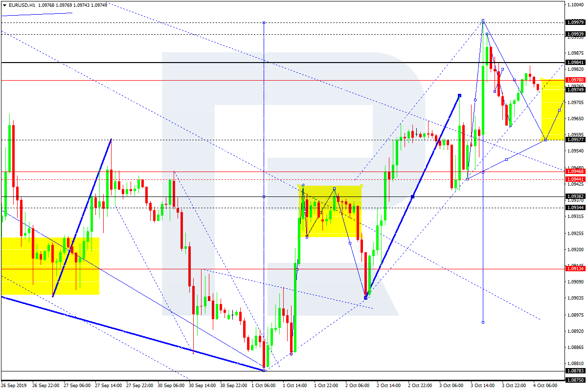
EURUSD has finished the ascending wave 1.0997; right now, it is forming the first descending impulse with the predicted target at 1.0957. Later, the market may start another correction to reach 1.0978, thus forming a new consolidation range between these two levels. After breaking this range to the downside, the instrument may continue trading inside the downtrend with the target at 1.0895.
GBPUSD, “Great Britain Pound vs US Dollar”
After breaking 1.2323, GBPUSD has reached 1.2400; right now, it is moving downwards. The target is at 1.2299. After that, the instrument may resume trading upwards with the target at 1.2355.
USDCHF, “US Dollar vs Swiss Franc”
USDCHF is moving upwards to reach 1.0018. Later, the market may form a new descending structure towards 0.9987 and then start another growth with the target at 1.0040.
USDJPY, “US Dollar vs Japanese Yen”
After breaking the consolidation range to the downside, USDJPY has reached 106.60. Possibly, today the pair may grow to break 107.25 and then continue moving upwards with the target at 108.00.
AUDUSD, “Australian Dollar vs US Dollar”
AUDUSD has broken the consolidation range to the upside; right now, it is still moving upwards to reach 0.6760. After that, the instrument may start a new decline towards 0.6730 and then continue trading upwards with the target at 0.6780.
USDRUB, “US Dollar vs Russian Ruble”
USDRUB is still consolidating above 65.00. Today, the pair may break 65.00 downwards. The first target is at 64.50. Later, the market may start a new correction to return to 65.00.
USDCAD, “US Dollar vs Canadian Dollar”
USDCAD is still consolidating above 1.3318. If later the price breaks this range to the downside, the instrument may start a new correction with the target at 1.3285; if to the upside – resume moving upwards to reach 1.3373.
XAUUSD, “Gold vs US Dollar”
Gold has completed the descending impulse; right now, it is consolidating around 1507.70. the main scenario implies that the pair may fall with the first target at 1496.50. Later, the market may start another correction towards 1507.50.
BRENT
Brent is moving upwards. Possibly, the pair may break 58.50. The first target is at 60.64. Later, the market may start another correction to return to 58.50 and then resume growing to reach 64.05.
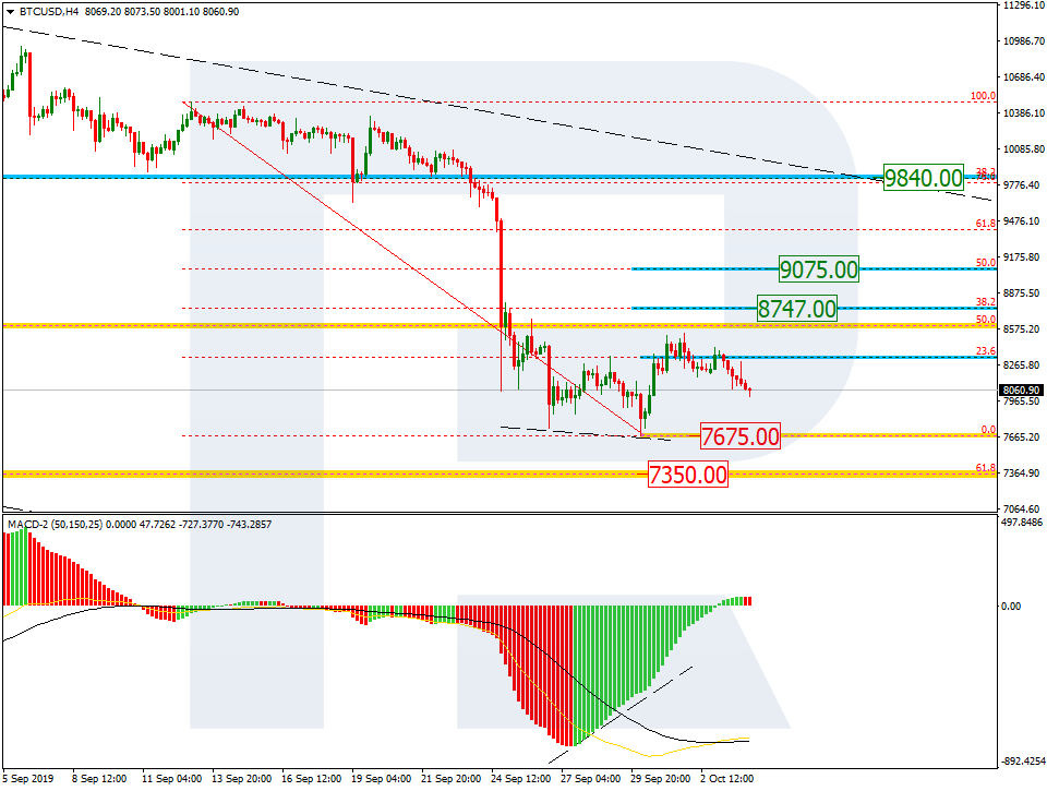
BTCUSD, “Bitcoin vs US Dollar”
BTCUSD has reached 8020.00. Possibly, today the pair may form one more ascending structure towards 8200.00, thus forming a new consolidation range between these two levels. If later the price breaks this range to the downside, the instrument may resume falling with the target at 7850.00; if to the upside – start another growth to reach 8400.00.
Attention! Forecasts presented in this section only reflect the author’s private opinion and should not be considered as guidance for trading. RoboForex LP bears no responsibility for trading results based on trading recommendations described in these analytical reviews.
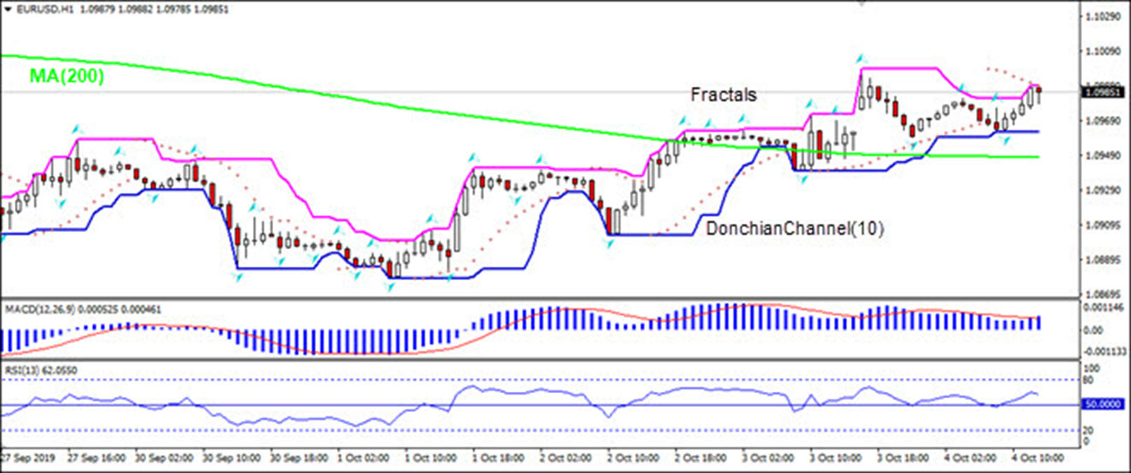
Producer Price Index for euro-zone declined 0.8% over year in August after 0.1% increase in July. Will the EURUSD decline?
The price chart on 1-hour timeframe shows EURUSD: H1 is trading sideways. The price is above the 200-period moving average MA(200) which is level. And the RSI is rising falling toward 50 level. There is no trend yet formed, traders have to decide when it would be a best time to enter the market.
As we can see in the H4 chart, the convergence made the pair complete a quick descending impulse and form a new correction. After reaching 23.6% fibo, the price started a pullback. Which may later be followed by further correction to the upside towards 38.2% and 50.0% fibo at 8747.00 and 9075.00 respectively. If the price breaks the low at 7675.00, BTCUSD will continue falling to reach the mid-term correctional target, 61.8% fibo at 7350.00.
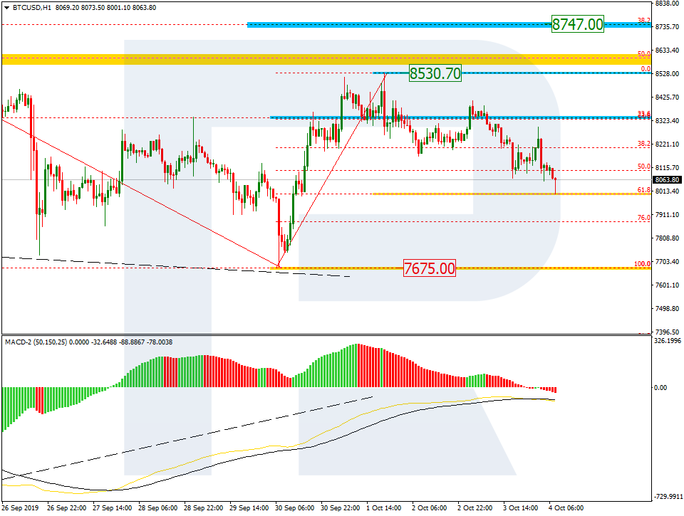
In the H1 chart, the current pullback has reached 61.8% fibo. In this case, the price is expected to start a new rising wave towards the high at 8530.70.
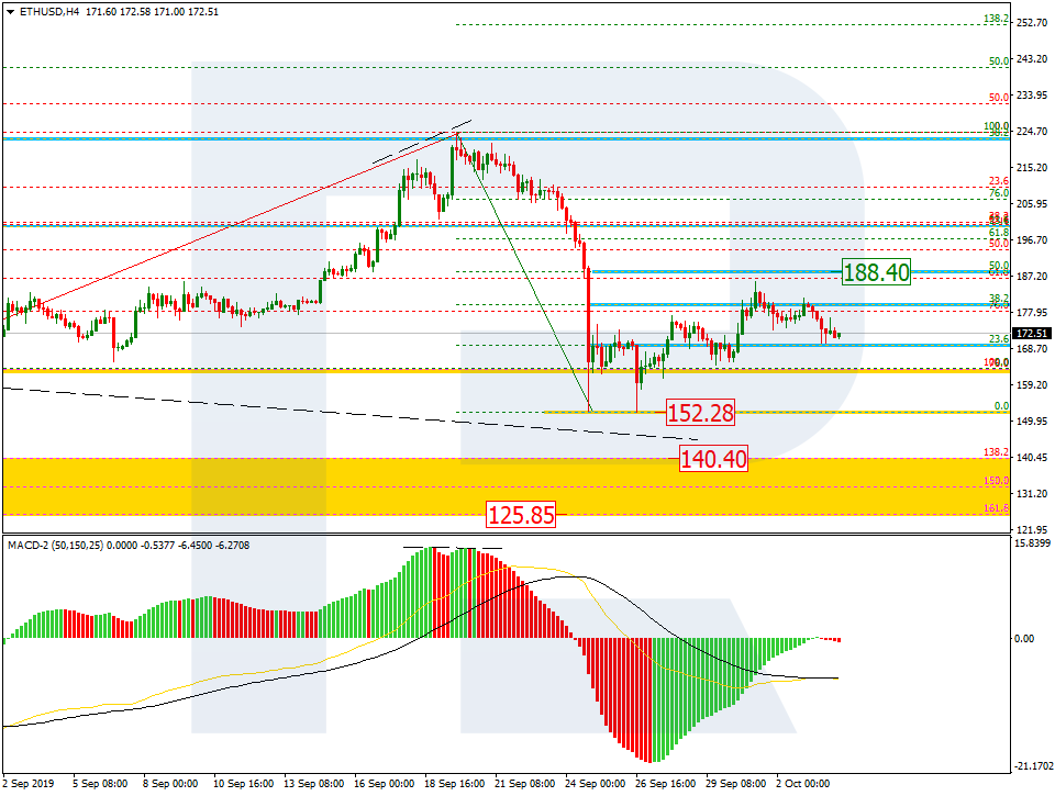
ETHUSD, “Ethereum vs. US Dollar”
As we can see in the H4 chart, ETHUSD has completed the ascending correction close to 50.0% fibo at 188.40. After breaking the low at 152.28, the instrument may start a new descending wave towards the post-correctional extension area between 138.2% and 161.8% fibo at 140.40 and 125.85 respectively.
In the H1 chart, the divergence on MACD made the pair start a new decline, which is getting close to 50.0% fibo at 169.00 and even 61.8% fibo at 165.08. If the price breaks the high at 185.78, the correction may yet continue.
Attention! Forecasts presented in this section only reflect the author’s private opinion and should not be considered as guidance for trading. RoboForex LP bears no responsibility for trading results based on trading recommendations described in these analytical reviews.
EUR/USD currency pair continues to show a positive trend. The trading tool again updated local highs. Greenback remains under pressure amid weak economic releases. In September, the ISM business activity index from the US non-manufacturing sector dropped to 52.6. Market expectations were at 55.0. At the moment, EUR/USD quotes are consolidating in the range 1.09650-1.09900. Financial market participants took a wait-and-see attitude before the publication of the US labor market report. We recommend that you pay attention to the difference between the actual and forecast values of the indicators. Positions must be opened from key levels.
At 15:30 (GMT+3:00), US will publish a labor statistics report for September.
Indicators signal the strength of buyers: the price has fixed above 50 MA and 100 MA.
The MACD histogram is in the positive zone, but below the signal line, which gives a weak signal to buy EUR/USD.
The Stochastic Oscillator is near the oversold zone, the %K line is below the %D line, which gives a weak signal to sell EUR/USD.
Trading recommendations
Support levels: 1.09650, 1.09400, 1.09050
Resistance levels: 1.09900, 1.10250
If the price consolidates above 1.09900, expect further growth toward 1.10250-1.10500.
Alternatively, the quotes could drop toward 1.09400-1.09200.
The GBP/USD currency pair
Technical indicators of the currency pair:
Prev Open: 1.22988
Open: 1.23288
% chg. over the last day: +0.33
Day’s range: 1.23288 – 1.23568
52 wk range: 1.1995 – 1.3385
Yesterday, purchases prevailed on the GBP/USD currency pair. Sterling set new local highs. Pressure on the USD continues to exert weak economic releases. Currently, GBP/USD quotes are consolidating in the range of 1.23200-1.23650. Today, investors will evaluate the report on the US labor market in September. We also recommend keeping track of up-to-date information regarding the Brexit process. Positions must be opened from key levels.
The Economic News Feed for 04.10.2019 is calm.
The price fixed above 50 MA and 100 MA, which signals the strength of buyers.
The MACD histogram is in the positive zone, but below the signal line, which gives a weak signal to buy GBP/USD.
The Stochastic Oscillator is in the neutral zone, the %K line crossed the %D line. There are no signals at the moment.
Trading recommendations
Support levels: 1.23200, 1.22600, 1.22100
Resistance levels: 1.23650, 1.24150, 1.24500
If the price consolidates above 1.23650, expect further recovery toward 1.24100-1.24400.
Alternatively, the quotes could retreat toward 1.22700-1.22500.
The USD/CAD currency pair
Technical indicators of the currency pair:
Prev Open: 1.33252
Open: 1.33330
% chg. over the last day: +0.11
Day’s range: 1.33243 – 1.33383
52 wk range: 1.2727 – 1.3664
The USD/CAD currency pair stabilized after a sharp rally the day before. Looney is currently consolidating. Unidirectional trends are not observed. The trading instrument formed the following local support and resistance levels: 1.33150 and 1.33450, respectively. Participants in financial markets expect the release of important statistics on the US and Canada economies. We recommend that you pay attention to the dynamics of prices of “black gold”. Positions must be opened from key levels.
The Economic News Feed for 04.10.2019:
– Ivey Canada Business Activity Index (CAD) – 17:00 (GMT+3:00);
Indicators signal the strength of buyers: the price has fixed above 50 MA and 100 MA.
The MACD histogram is in the positive zone, but below the signal line, which gives a weak signal to buy USD/CAD.
The Stochastic Oscillator is in the neutral zone, the% K line began to cross the% D line. There are no signals at the moment.
Trading recommendations
Support levels: 1.33150, 1.33000, 1.32800
Resistance levels: 1.33450, 1.33700, 1.34000
If the price consolidates above 1.33450, expect further growth toward 1.33700-1.34000.
Alternatively, the quotes could decrease toward 1.32800-1.32600.
The USD/JPY currency pair
Technical indicators of the currency pair:
Prev Open: 107.178
Open: 106.913
% chg. over the last day: -0.33
Day’s range: 106.744 – 106.924
52 wk range: 104.97 – 114.56
The USD/JPY currency pair is still dominated by bearish sentiment. The trading tool again updated local lows. At the moment, USD/JPY quotes are consolidating in the range of 106.700 and 107.000, respectively. The focus is on the US labor market report. We recommend that you keep track of up-to-date information regarding trade negotiations between Washington and Beijing. Positions must be opened from key levels.
The Economic News Feed for 04.10.2019 is calm.
Indicators signal the strength of sellers: the price has fixed below 50 MA and 100 MA.
The MACD histogram is in the negative zone, but above the signal line, which gives a weak signal to sell USD/JPY.
The Stochastic Oscillator is in the neutral zone, the% K line is above the% D line, which indicates bullish sentiment.
Trading recommendations
Support levels: 106.700, 106.500
Resistance levels: 107.000, 107.350, 107.650
If the price consolidates below 106.700, expect a drop toward 106.400-106.200.
Alternatively, the quotes could grow toward 107.300-107.000.
In this article we look at an interesting data problem – making decisions about the algorithms used for image segmentation, or separating one qualitatively different part of an image from another.
Example code for this article may be found at the Kite Github repository. We have provided tips on how to use the code throughout.
As our example, we work through the process of differentiating vascular tissue in images, produced by Knife-edge Scanning Microscopy (KESM). While this may seem like a specialized use-case, there are far-reaching implications, especially regarding preparatory steps for statistical analysis and machine learning.
Data scientists and medical researchers alike could use this approach as a template for any complex, image-based data set (such as astronomical data), or even large sets of non-image data. After all, images are ultimately matrices of values, and we’re lucky to have an expert-sorted data set to use as ground truth. In this process, we’re going to expose and describe several tools available via image processing and scientific Python packages (opencv, scikit-image, and scikit-learn). We’ll also make heavy use of the numpy library to ensure consistent storage of values in memory.
The procedures we’ll explore could be used for any number of statistical or supervised machine learning problems, as there are a large number of ground truth data points. In order to choose our image segmentation algorithm and approach, we will demonstrate how to visualize the confusion matrix, using matplotlib to colorize where the algorithm was right and where it was wrong. In early stages, it’s more useful for a human to be able to clearly visualize the results than to aggregate them into a few abstract numerals.
Approach
Cleaning
To remove noise, we use a simple median filter to remove the outliers, but one can use a different noise removal approach or artifact removal approach. The artifacts vary across acquisition systems (microscopy techniques) and may require complicated algorithms to restore the missing data. Artifacts commonly fall into two categories:
blurry or out-of-focus areas
imbalanced foreground and background (correct with histogram modification)
Segmentation
For this article, we limit segmentation to Otsu’s approach, after smoothing an image using a median filter, followed by validation of results. You can use the same validation approach for any segmentation algorithm, as long as the segmentation result is binary. These algorithms include, but are not limited to, various Circular Thresholding approaches that consider different color space.
Some examples are:
Li Thresholding
An adaptive thresholding method that is dependent on local intensity
Deep learning algorithms like UNet used commonly in biomedical image segmentation
Deep learning approaches that semantically segment an image
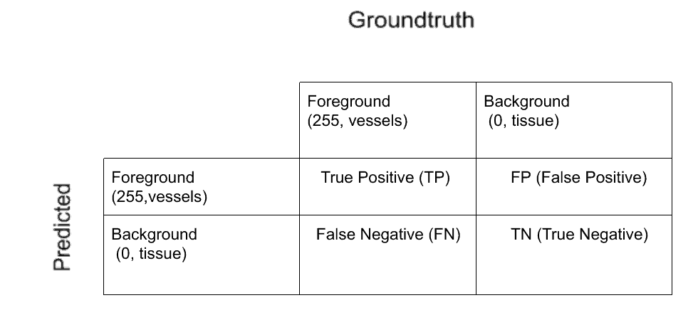
Validation
We begin with a ground truth data set, which has already been manually segmented. To quantify the performance of a segmentation algorithm, we compare ground truth with the predicted binary segmentation, showing accuracy alongside more effective metrics. Accuracy can be abnormally high despite a low number of true positives (TP) or false negatives (FN). In such cases, F1 Score and MCC are better quantification metrics for the binary classification.We’ll go into detail on the pros and cons of these metrics later.
For qualitative validation, we overlay the confusion matrix results i.e where exactly the true positives, true negatives, false positives, false negatives pixels are onto the grayscale image. This validation can also be applied to a color image on a binary image segmentation result, although the data we used in this article is a grayscale image. In the end, we will present the whole process so that you can see the results for yourself. Now, let’s look at the data–and the tools used to process that data.
Loading and visualizing data
We will use the below modules to load, visualize, and transform the data. These are useful for image processing and computer vision algorithms, with simple and complex array mathematics. The module names in parentheses will help if installing individually.
Module
Reason
numpy
Histogram calculation, array math, and equality testing
matplotlib
Graph plotting and Image visualization
scipy
Image reading and median filter
cv2 (opencv-python)
Alpha compositing to combine two images
skimage (scikit-image)
Image thresholding
sklearn (scikit-learn)
Binary classifier confusion matrix
nose
Testing
Displaying Plots Sidebar: If you are running the example code in sections from the command line, or experience issues with the matplotlib backend, disable interactive mode by removing the plt.ion() call, and instead call plt.show() at the end of each section, by uncommenting suggested calls in the example code. Either ‘Agg’ or ‘TkAgg’ will serve as a backend for image display. Plots will be displayed as they appear in the article.
Importing modules
import cv2
import matplotlib.pyplot as plt
import numpy as np
import scipy.misc
import scipy.ndimage
import skimage.filters
import sklearn.metrics

# Turn on interactive mode. Turn off with plt.ioff()
plt.ion()
In this section, we load and visualize the data. The data is an image of mouse brain tissue stained with India ink, generated by Knife-Edge Scanning Microscopy (KESM). This 512 x 512 image is a subset, referred to as a tile. The full data set is 17480 x 8026 pixels, 799 slices in depth, and 10gb in size. So, we will write algorithms to process the tile of size 512 x 512 which is only 150 KB.
Individual tiles can be mapped to run on multi processing/multi threaded (i.e. distributed infrastructure), and then stitched back together to obtain the full segmented image. The specific stitching method is not demonstrated here. Briefly, stitching involves indexing the full matrix and putting the tiles back together according to this index. For combining numerical values, you can use map-reduce. Map-Reduce yields metrics such as the sum of all the F1 scores along all tiles, which you can then average. Simply append the results to a list, and then perform your own statistical summary.
The dark circular/elliptical disks on the left are vessels and the rest is the tissue. So, our two classes in this dataset are:
foreground (vessels) – labeled as 255
background (tissue) – labeled as 0
The last image on the right below is the ground truth image. Vessels are traced manually by drawing up contours and filling them to obtain the ground truth by a board-certified pathologist. We can use several examples like these from experts to train supervised deep learning networks and validate them on a larger scale. We can also augment the data by giving these examples to crowdsourced platforms and training them to manually trace a different set of images on a larger scale for validation and training. The image in the middle is just an inverted grayscale image, which corresponds with the ground truth binary image.
Before segmenting the data, you should go through the dataset thoroughly to determine if there are any artifacts due to the imaging system. In this example, we only have one image in question. By looking at the image, we can see that there aren’t any noticeable artifacts that would interfere with the segmentation. However, you can remove outlier noise and smooth an image using a median filter. A median filter replaces the outliers with the median (within a kernel of a given size).
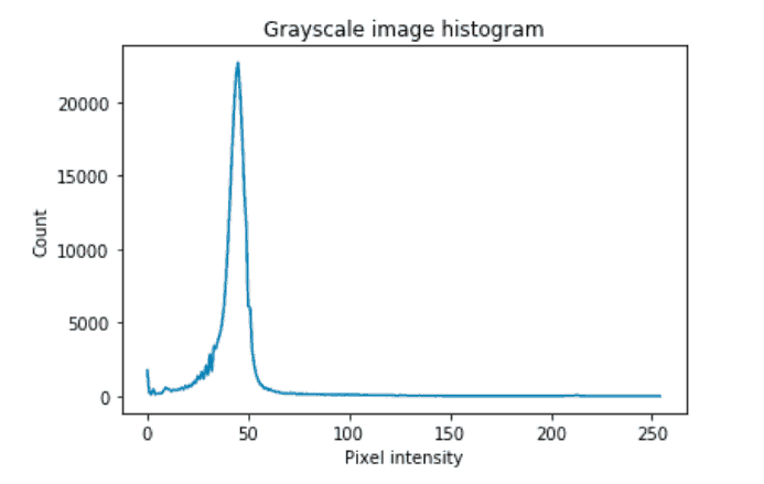
To determine which thresholding technique is best for segmentation, you could start by thresholding to determine if there is a distinct pixel intensity that separates the two classes. In such cases, you can use that intensity obtained by the visual inspection to binarize the image. In our case, there seem to be a lot of pixels with intensities of less than 50 which correspond to the background class in the inverted grayscale image.
Although the distribution of the classes is not bimodal (having two distinct peaks), it still has a distinction between foreground and background, which is where the lower intensity pixels peak and then hit a valley. This exact value can be obtained by various thresholding techniques. The segmentation section examines one such method in detail.
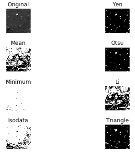
After removing noise, you can apply the skimage filters module to try all thresholds to explore which thresholding methods fare well. Sometimes, in an image, a histogram of its pixel intensities is not bimodal. So, there might be another thresholding method that can fare better like an adaptive thresholding method that does thresholding based on local pixel intensities within a kernel shape. It’s good to see what the different thresholding methods results are, and skimage.filters.thresholding.try_all_threshold() is handy for that.
Try all thresholding method
result = skimage.filters.thresholding.try_all_threshold(median_filtered)
The simplest thresholding approach uses a manually set threshold for an image. On the other hand, using an automated threshold method on an image calculates its numerical value better than the human eye and may be easily replicated. For our image in this example, it seems like Otsu, Yen, and the Triangle method are performing well. The other results for this case are noticeably worse.
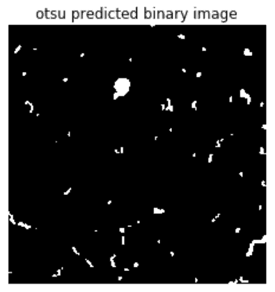
We’ll use the Otsu thresholding to segment our image into a binary image for this article. Otsu calculates thresholds by calculating a value that maximizes inter-class variance (variance between foreground and background) and minimizes intra-class variance (variance within foreground or variance within background). It does well if there is either a bimodal histogram (with two distinct peaks) or a threshold value that separates classes better.
If the above simple techniques don’t serve the purpose for binary segmentation of the image, then one can use UNet, ResNet with FCN or various other supervised deep learning techniques to segment the images. To remove small objects due to the segmented foreground noise, you may also consider trying skimage.morphology.remove_objects().
Validation
In any of the cases, we need the ground truth to be manually generated by a human with expertise in the image type to validate the accuracy and other metrics to see how well the image is segmented.
The confusion matrix
We use sklearn.metrics.confusion_matrix() to get the confusion matrix elements as shown below. Scikit-learn confusion matrix function returns 4 elements of the confusion matrix, given that the input is a list of elements with binary elements. For edge cases where everything is one binary value(0) or other(1), sklearn returns only one element. We wrap the sklearn confusion matrix function and write our own with these edge cases covered as below:
get_confusion_matrix_elements()
defget_confusion_matrix_elements(groundtruth_list, predicted_list):"""returns confusion matrix elements i.e TN, FP, FN, TP as floats
See example code for helper function definitions
"""
_assert_valid_lists(groundtruth_list, predicted_list)
if _all_class_1_predicted_as_class_1(groundtruth_list, predicted_list) isTrue:
tn, fp, fn, tp = 0, 0, 0, np.float64(len(groundtruth_list))
elif _all_class_0_predicted_as_class_0(groundtruth_list, predicted_list) isTrue:
tn, fp, fn, tp = np.float64(len(groundtruth_list)), 0, 0, 0else:
tn, fp, fn, tp = sklearn.metrics.confusion_matrix(groundtruth_list, predicted_list).ravel()
tn, fp, fn, tp = np.float64(tn), np.float64(fp), np.float64(fn), np.float64(tp)
return tn, fp, fn, tp
Accuracy
Accuracy is a common validation metric in case of binary classification. It is calculated as
It varies between 0 to 1, with 0 being the worst and 1 being the best. If an algorithm detects everything as either entirely background or foreground, there would still be a high accuracy. Hence we need a metric that considers the imbalance in class count. Especially since the current image has more foreground pixels(class 1) than background 0.
F1 score
The F1 score varies from 0 to 1 and is calculated as:
with 0 being the worst and 1 being the best prediction. Now let’s handle F1 score calculation considering edge cases.
An F1 score of above 0.8 is considered a good F1 score indicating prediction is doing well.
MCC
MCC stands for Matthews Correlation Coefficient, and is calculated as:
It lies between -1 and +1. -1 is absolutely an opposite correlation between ground truth and predicted, 0 is a random result where some predictions match and +1 is where absolutely everything matches between ground and prediction resulting in positive correlation. Hence we need better validation metrics like MCC.
In MCC calculation, the numerator consists of just the four inner cells (cross product of the elements) while the denominator consists of the four outer cells (dot product of the) of the confusion matrix. In the case where the denominator is 0, MCC would then be able to notice that your classifier is going in the wrong direction, and it would notify you by setting it to the undefined value (i.e. numpy.nan). But, for the purpose of getting valid values, and being able to average the MCC over different images if necessary, we set the MCC to -1, the worst possible value within the range. Other edge cases include all elements correctly detected as foreground and background with MCC and F1 score set to 1. Otherwise, MCC is set to -1 and F1 score is 0.
To learn more about MCC and the edge cases, this is a good article. To understand why MCC is better than accuracy or F1 score more in detail, Wikipedia does good work here.
Accuracy is close to 1, as we have a lot of background pixels in our example image that are correctly detected as background (i.e. true negatives are are naturally higher). This shows why accuracy isn’t a good measure for binary classification.
F1 score is 0.84. So, in this case, we probably don’t need a more sophisticated thresholding algorithm for binary segmentation. If all the images in the stack had similar histogram distribution and noise, then we could use Otsu and have satisfactory prediction results.
The MCC of 0.85 is high, also indicating the ground truth and predicted image have a high correlation, clearly seen from the predicted image picture from the previous section.
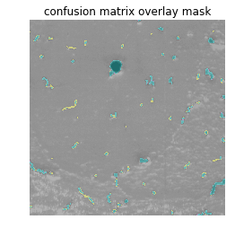
Now, let’s visualize and see where the confusion matrix elements TP, FP, FN, TN are distributed along the image. It shows us where the threshold is picking up foreground (vessels) when they are not present (FP) and where true vessels are not detected (FN), and vice-versa.
Validation visualization
To visualize confusion matrix elements, we figure out exactly where in the image the confusion matrix elements fall. For example, we find the TP array (i.e. pixels correctly detected as foreground) is by finding the logical “and” of the ground truth and the predicted array. Similarly, we use logical boolean operations commonly called as Bit blit to find the FP, FN, TN arrays.
Then, we can map pixels in each of these arrays to different colors. For the figure below we mapped TP, FP, FN, TN to the CMYK (Cyan, Magenta, Yellow, Black) space. One could similarly also map them to (Green, Red, Red, Green) colors. We would then get an image where everything in red signifies the incorrect predictions. The CMYK space allows us to distinguish between TP, TN.
get_confusion_matrix_overlaid_mask()
defget_confusion_matrix_overlaid_mask(image, groundtruth, predicted, alpha, colors):"""
Returns overlay the 'image' with a color mask where TP, FP, FN, TN are
each a color given by the 'colors' dictionary
"""
image = cv2.cvtColor(image, cv2.COLOR_GRAY2RGB)
masks = get_confusion_matrix_intersection_mats(groundtruth, predicted)
color_mask = np.zeros_like(image)
for label, mask in masks.items():
color = colors[label]
mask_rgb = np.zeros_like(image)
mask_rgb[mask != 0] = color
color_mask += mask_rgb
return cv2.addWeighted(image, alpha, color_mask, 1 - alpha, 0)
alpha = 0.5
confusion_matrix_colors = {
'tp': (0, 255, 255), #cyan'fp': (255, 0, 255), #magenta'fn': (255, 255, 0), #yellow'tn': (0, 0, 0) #black
}
validation_mask = get_confusion_matrix_overlaid_mask(255 - grayscale, groundtruth, predicted, alpha, confusion_matrix_colors)
print('Cyan - TP')
print('Magenta - FP')
print('Yellow - FN')
print('Black - TN')
plt.imshow(validation_mask)
plt.axis('off')
plt.title('confusion matrix overlay mask')
We use opencv here to overlay this color mask onto the original (non-inverted) grayscale image as a transparent layer. This is called Alpha compositing:
Final notes
The last two examples in the repository are testing the edge cases and a random prediction scenario on a small array (fewer than 10 elements), by calling the test functions. It is important to test for edge cases and potential issues if we are writing production level code, or just to test the simple logic of an algorithm.
Travis CI is very useful for testing whether your code works on the module versions described in your requirements, and if all the tests pass as new changes are merged into master. Keeping your code clean, well documented, and with all statements unit tested and covered is a best practice. These habits limit the need to chase down bugs, when a complex algorithm is built on top of simple functional pieces that could have been unit tested. Generally, documentation and unit testing helps others stay informed about your intentions for a function. Linting helps improve readability of the code, and flake8 is good Python package for that.
Here are the important takeaways from this article:
Tiling and stitching approach for data that doesn’t fit in memory
Trying different thresholding techniques
Subtleties of Validation Metrics
Validation visualization
Best Practices
There are many directions you could go from here with your work or projects. Applying the same strategy to different data sets, or automating the validation selection approach would be excellent places to start. Further, imagine you needed to analyze a database with many of these 10gb files. How could you automate the process? How could you validate and justify the results to human beings? How does better analysis improve the outcomes of real-world scenarios (like the development of surgical procedures and medicine)? Asking questions like these will allow continued improvements in Statistics, Data Science, and Machine Learning.
Finally, Thanks to Navid Farahani for annotations, Katherine Scott for the guidance, Allen Teplitsky for the motivation, and all of the 3Scan team for the data.